pacman::p_load(jsonlite,tidygraph, ggraph, visNetwork, tidyverse,igraph, lubridate, clock,tidyverse, graphlayouts,plotly)Take-home Exercise 2
Take home exercise 2
The task
With reference to Mini-Challenge 2 of VAST Challenge 2023 and by using appropriate static and interactive statistical graphics methods, you are required to help FishEye identify companies that may be engaged in illegal fishing. (website: https://vast-challenge.github.io/2023/MC2.html)
Question chosen: Use visual analytics to identify temporal patterns for individual entities and between entities in the knowledge graph FishEye created from trade records. Categorize the types of business relationship patterns you find.
Data pre-processing
load packages and read datasets
MC2 <- jsonlite::fromJSON("D:/MITB/ISSS608/fruitpunchsamurai666/website/Take-home_EX/Take-home_EX02/data/mc2_challenge_graph.json")read nodes and edge from JSON
#read the sub-dataframe from the json file, select and rearrange the columns needed
mc2_nodes <- as_tibble(MC2$nodes) %>%
  select(id, shpcountry, rcvcountry)
mc2_edges <- as_tibble(MC2$links) %>%
  mutate(ArrivalDate = ymd(arrivaldate)) %>%
  mutate(Year = year(ArrivalDate)) %>%
  select(source, target, ArrivalDate, Year, hscode, valueofgoods_omu,
         volumeteu, weightkg, valueofgoodsusd) %>%
  distinct()
Wrangling attributes by grouping by source-target-year pair, and record the count as weight (only interested in those with count >100).
The HS code is composed of six digits, which provide information about the classification of goods. Research suggests that the first two digits of the hscode represent the chapter. The next two digits represent the heading. The following two digits indicate the subheading. In this exercise, I only keep rows with hscode starting with “30” or “16” which is custom Duty Of Fish and crustaceans/molluscs/other aquatic invertebrates and custom Duty Of preparation of meat/fish/crustaceans/molluscs/other aquatic invertebrates respectively. (Reference: https://www.cybex.in/indian-custom-duty/)
    #filter out edges with first 2 characters of hscodes = 30 or 16, aggregate and keep count >100 ones
    mc2_edges_aggregated <- mc2_edges %>%
      filter(substr(hscode, 1, 2) == "30"|substr(hscode, 1, 2) == "16") %>%
      group_by(source, target, Year) %>%
        summarise(weights = n()) %>%
      filter(source!=target) %>%
      filter(weights > 100) %>%   #only keep those with count >100
      ungroup()

    #update nodes list according to the updated edge list
    id1 <- mc2_edges_aggregated %>%
      select(source) %>%
      rename(id = source)
    id2 <- mc2_edges_aggregated %>%
      select(target) %>%
      rename(id = target)
    mc2_nodes_extracted <- rbind(id1, id2) %>%
      distinct()
Visualize the distribution of hscode chapters to understand the proportions of fishing related transactions.
Show Code
  counts <- mc2_edges %>%
        group_by(chapter=substr(hscode, 1, 2)) %>%
        summarise(weights = n()) %>%
        ungroup()

  total <- sum(counts$weights)
  counts$percentage <- (counts$weights/ total) * 100

  highlight_chapter <- c("30","16")

  hscode_hist <- ggplot(data= counts,
         aes(x= reorder(chapter,-percentage),y=percentage)) +
    #geom_bar(stat = "identity",fill= '#6eba6a')   +
    geom_bar(aes(fill = chapter %in% highlight_chapter), stat = "identity")+
    geom_text(aes(label = ifelse(chapter %in% highlight_chapter, chapter, "")),
              vjust = -0.5, color = "black", size = 3) +
    labs(y= 'No. of records', x= 'chapter',
         subtitle = "Distribution of hscode") +
    scale_fill_manual(values = c("steelblue", "orange"), guide = FALSE) +
    theme(axis.title.y= element_text(angle=0), axis.text.x = element_blank(),
          panel.background= element_blank(), axis.line= element_line(color= 'dimgrey'),
          plot.subtitle = element_text(color = "dimgrey", size = 12, face = "bold", hjust=0.5))
  hscode_hist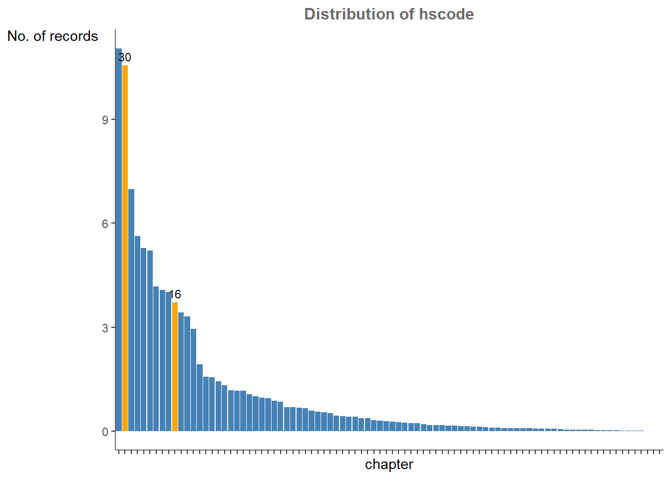
- Build network graph dataframe.
    mc2_graph <- tbl_graph(nodes = mc2_nodes_extracted,
                           edges = mc2_edges_aggregated,
directed = TRUE)- Have a quick view of the network.
Show Code
      ggraph(mc2_graph,
           layout = "fr") +
      geom_edge_link(arrow = arrow(length = unit(2, 'mm'))) +
      geom_node_point(aes()) +
      theme_graph()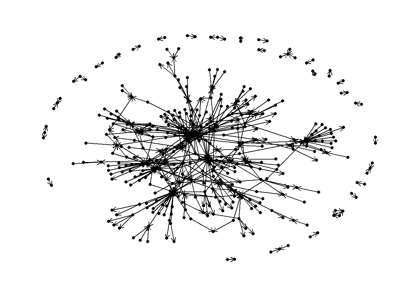
- The plot above is too dense. Now let us view the network by year.
Show Code
    set_graph_style()

    g <- ggraph(mc2_graph,
                layout = "nicely") +
      geom_edge_link(aes(width=weights),
                     alpha=0.2,arrow = arrow(length = unit(3, 'mm'))) +
      scale_edge_width(range = c(0.1, 5)) +
      geom_node_point( aes(),
                      size = 1)

    g + facet_edges(~Year) +
      th_foreground(foreground = "grey80",
                    border = TRUE) +
      theme(legend.position = 'bottom')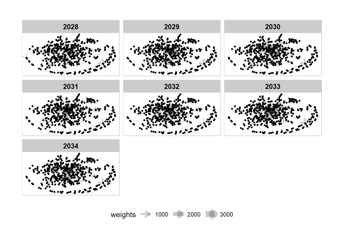
- It is still hard to visualize difference of the network plot by year. To be able to further zoom into the network, I decided to use the interactive visNetwork tool to better visualize it.
Firstly create a function that can filter out edges from a specific year with trading records > 100 (similar to the previous step).
Show Code
  mc2_subset <- function(mc2_edges,year) {
    mc2_edges_aggregated <- mc2_edges %>%
    filter(Year == year) %>%
    filter(substr(hscode, 1, 2) == "30"|substr(hscode, 1, 2) == "16") %>%
    group_by(source, target, Year) %>%
      summarise(weights = n()) %>%
    filter(source!=target) %>%
    filter(weights > 100) %>%
    ungroup()

    #change column names for visnetwork usage later
    colnames(mc2_edges_aggregated) <- c("from", "to", "Year", "weights")
    return(mc2_edges_aggregated)
  }
Then create another function that can update the unique nodes according to the edges subset by year (similar to the previous step).
Show Code
  update_nodes <- function(mc2_edges_aggregated) {
    id1 <- mc2_edges_aggregated %>%
     select(from) %>%
     rename(id = from)
    id2 <- mc2_edges_aggregated %>%
     select(to) %>%
      rename(id = to)
    mc2_nodes_extracted <- rbind(id1, id2) %>%
      distinct()
    return(mc2_nodes_extracted)
  }
Pass the filtered edge data into the function to generate a subset for each year, then generate the node list for that year accordingly as well.
Show Code
  edges_2028 <- mc2_subset(mc2_edges,2028)
  nodes_2028 <- update_nodes(edges_2028)

  edges_2029 <- mc2_subset(mc2_edges,2029)
  nodes_2029 <- update_nodes(edges_2029)

  edges_2030 <- mc2_subset(mc2_edges,2030)
  nodes_2030 <- update_nodes(edges_2030)

  edges_2031 <- mc2_subset(mc2_edges,2031)
  nodes_2031 <- update_nodes(edges_2031)

  edges_2032 <- mc2_subset(mc2_edges,2032)
  nodes_2032 <- update_nodes(edges_2032)

  edges_2033 <- mc2_subset(mc2_edges,2033)
  nodes_2033 <- update_nodes(edges_2033)

  edges_2034 <- mc2_subset(mc2_edges,2034)
  nodes_2034 <- update_nodes(edges_2034)
Community Detection
I use “louvain_partition” to detect the communities within the subset of each year, and observe how they evolve over time. (One limitation is that multi-level community detection works for undirected graphs only, so in this section mc2_graph directed is set to false).
Show Code
#return top 5 nodes with the highest degree for big communities (with nodes > 10)
top_5  <- function(nodes,edges) {
  mc2_graph <- tbl_graph(nodes = nodes,
                         edges = edges,
                         directed = FALSE)
  set.seed(123)
  # run louvain with edge weights
  louvain_partition <- igraph::cluster_louvain(mc2_graph, weights = E(mc2_graph)$weights)

  # assign communities to graph
  mc2_graph$community <- louvain_partition$membership

  top_five <- data.frame()
  for (i in unique(mc2_graph$community)) {

    # create subgraph for each community
    subgraph <- induced_subgraph(mc2_graph, v = which(mc2_graph$community == i))

    # for larger communities
    if (igraph::gorder(subgraph) > 10) {  # only interested in big communities with nodes >10
      # get degree
      degree <- igraph::degree(subgraph)

      # get top five degrees
     top_indices <- head(order(degree, decreasing = TRUE), 5)
     top <- V(subgraph)$id[top_indices]
    result <- data.frame(community = rep(i, length(top)), rank = 1:5, character = top)
    } else {
      result <- data.frame(community = NULL, rank = NULL, character = NULL)
    }

    top_five <- top_five %>%
      dplyr::bind_rows(result)
  }
  return(top_five)
}
For big communities (with nodes > 10), return companies with top 5 highest degree centrality to investigate the changes over the year.
Show Code
top2028 <- top_5(nodes_2028,edges_2028)
top2029 <- top_5(nodes_2029,edges_2029)
top2030 <- top_5(nodes_2030,edges_2030)
top2031 <- top_5(nodes_2031,edges_2031)
top2032 <- top_5(nodes_2032,edges_2032)
top2033 <- top_5(nodes_2033,edges_2033)
top2034 <- top_5(nodes_2034,edges_2034)

knitr::kable(
top2028 %>%
  tidyr::pivot_wider(names_from = rank, values_from = character),
  caption = "2028 - companies with top 5 degree centrality in big communities"
)| community | 1 | 2 | 3 | 4 | 5 |
|---|---|---|---|---|---|
| 1 | Caracola del Sol Services | Pao gan SE Seal | Greek Octopus SRL Logistics | Manipur Market Corporation Cargo | Náutica del Mar Barracuda |
| 5 | hǎi dǎn Corporation Wharf | Mar de la Costa Company | Goa Seaside Sp Overseas | Marine Mermaids Incorporated Services | Nagaland Sea OJSC United |
| 11 | Mar del Este CJSC | Danish Plaice Swordfish AB Shipping | Assam Market GmbH & Co. KG Dockyard | Cape of Good Hope Corporation | Diao yu BV Logistics |
| 21 | Mar de la Felicidad Corporation | Punjab s Marine conservation | bǐ mù yú Sagl Distribution | Yu xian SRL Industrial | Pao gan LC Freight |
Show Code
knitr::kable(
top2029 %>%
  tidyr::pivot_wider(names_from = rank, values_from = character),
  caption = "2029 - companies with top 5 degree centrality in big communities"
)| community | 1 | 2 | 3 | 4 | 5 |
|---|---|---|---|---|---|
| 10 | hǎi dǎn Corporation Wharf | Madhya Pradesh Market LLC | Marine Mermaids Incorporated Services | Sea Star LLC Shipping | Rift Valley fishery Inc |
| 13 | Selous Game Reserve S.A. de C.V. | Chuan gou N.V. Delivery | Neptune’s Harvest A/S Hijiki | Lake Tanganyika Inc Jetty | Pregolya S.A. de C.V. Import |
| 19 | Uttarakhand Market Limited Liability Company Nautical | Náutica del Sol Brothers | Seaside Summit SE Merchants | Volga River LLC Enterprises | Estrella de la Costa SRL |
Show Code
knitr::kable(
top2030 %>%
  tidyr::pivot_wider(names_from = rank, values_from = character),
  caption = "2030 - companies with top 5 degree centrality in big communities"
)| community | 1 | 2 | 3 | 4 | 5 |
|---|---|---|---|---|---|
| 2 | Mar del Este CJSC | Sea Breeze Corporation Marine sanctuary | Chuan gou N.V. Delivery | Olas del Mar N.V. | Wave Watchers Ltd. Liability Co |
| 5 | Costa de la Felicidad Shipping | Baltic Catch SE Solutions | Blue Horizon Family & | Mar del Paraíso Corporation Logistics | Madagascar Coast AG Freight |
| 8 | Yu gan Sea spray GmbH Industrial | Arena del Sol SRL | Assam Market GmbH & Co. KG Dockyard | Cape of Good Hope Corporation | David Limited Liability Company Worldwide |
| 14 | Caracola del Sol Services | Kong zhong diao yu Ges.m.b.H. | Sea Breezes S.A. de C.V. Freight | Náutica del Mar Barracuda | Océano de Coral Corporation Marine conservation |
Show Code
knitr::kable(
top2031 %>%
  tidyr::pivot_wider(names_from = rank, values_from = character) ,
  caption = "2031 - companies with top 5 degree centrality in big communities"
)| community | 1 | 2 | 3 | 4 | 5 |
|---|---|---|---|---|---|
| 5 | Mar del Este CJSC | Chuan gou N.V. Delivery | Wave Watchers Ltd. Liability Co | Sea Breeze Corporation Marine sanctuary | Aqua Aura Nori Ltd. Corporation Brothers |
| 13 | Caracola del Sol Services | Sea Breezes S.A. de C.V. Freight | Kong zhong diao yu Ges.m.b.H. | Costa de Oro BV | Costa de Oro CJSC |
Show Code
knitr::kable(
top2032 %>%
  tidyr::pivot_wider(names_from = rank, values_from = character) ,
  caption = "2032 - companies with top 5 degree centrality in big communities"
)| community | 1 | 2 | 3 | 4 | 5 |
|---|---|---|---|---|---|
| 1 | Caracola del Sol Services | Sea Breezes S.A. de C.V. Freight | Pao gan SE Seal | Playa de Arena OJSC Express | Caracola del Este Ltd. Liability Co |
| 5 | Mar del Este CJSC | Aqua Aura Nori Ltd. Corporation Brothers | Chuan gou N.V. Delivery | Costa de Coral SRL United | Danish Plaice Swordfish AB Shipping |
| 10 | Costa de la Felicidad Shipping | Blue Horizon Family & | Daniel Ferry N.V. Transit | Madagascar Coast AG Freight | Barco de Plata CJSC |
Show Code
knitr::kable(
top2033 %>%
  tidyr::pivot_wider(names_from = rank, values_from = character) ,
  caption = "2033 - companies with top 5 degree centrality in big communities"
)| community | 1 | 2 | 3 | 4 | 5 |
|---|---|---|---|---|---|
| 2 | Caracola del Sol Services | Playa de Arena OJSC Express | Pao gan LC Freight | Spanish Shrimp A/S Marine | Caracola del Este Ltd. Liability Co |
| 8 | Mar del Este CJSC | Blue Horizon Family & | Lake Tana & Son’s | Costa de la Felicidad Shipping | Madagascar Coast AG Freight |
| 11 | Kong zhong diao yu Ges.m.b.H. | AquaDelight N.V. Coral Reef | Estrella de la Costa SRL | Dutch Eel AB Holdings | Marit GmbH & Co. KG |
| 13 | Pao gan SE Seal | Kilimajaro Slopes Incorporated and Son’s | Sea Breezes S.A. de C.V. Freight | nián yú Ltd. Corporation | Arena del Mar Marine Marine biology |
Show Code
knitr::kable(
top2034 %>%
  tidyr::pivot_wider(names_from = rank, values_from = character) ,
  caption = "2034 - companies with top 5 degree centrality in big communities"
)| community | 1 | 2 | 3 | 4 | 5 |
|---|---|---|---|---|---|
| 2 | Belgian Cod BV Solutions | David Limited Liability Company Worldwide | Angeline Sea NV Worldwide | Blue Horizon Inc Transport | Cape of Good Hope Corporation |
| 4 | hǎi dǎn Corporation Wharf | Aqua Aura SE Marine life | Balkan Cat ОАО Transport | Gambia River Ges.m.b.H. & | LLC S.A. de C.V. |
| 7 | Mar del Este CJSC | Neptune’s Harvest A/S Hijiki | Estrella de la Costa AB Express | Seaside Summit SE Merchants | Belgian Scallop Harbor ОАО Freight |
| 9 | AquaDelight N.V. Coral Reef | Madagascar Coast AG Freight | Estrella de la Costa SRL | Lake Tana & Son’s | Estrella del Mar Tilapia Oyj Marine |
| 10 | Olas del Sur Ltd | Uttarakhand Tidepool Oyj International | Cape Verde Islands Sp Transportation | Manipur Market Ltd. Liability Co | Manipur Market Ltd. Liability Co Transport |
| 14 | Pao gan SE Seal | nián yú Ltd. Corporation | Arena del Mar Marine Marine biology | Niger Bend Limited Liability Company Marine ecology | Kilimajaro Slopes Incorporated and Son’s |
From the table we can see that “Sea Breezes S.A. de C.V. Freight” company became one of the companies with highest degree since 2030 and its degree centrality remains high for a few years. This could be a possible sign of illegal fishing.
From the names of the company, we can see that there are some companies seem to have same origin and have their business extended in several different big communities. This might suggest some black market activities. For example:
Pao gan LC Freight & Pao gan SE Seal (community 2 and 13 in year 2033)
Estrella de la Costa AB Express & Estrella de la Costa SRL & Estrella del Mar Tilapia Oyj Marine (community 7 and 9 in year 2034)
Network Evolution
Plot interactive visNetwork for each year, color the nodes by the community (group) detected. Node size indicates the betweenness centrality value. Edge width indicates the number of transactions between the two nodes.
Show Code
plot <- function(nodess,edgess,years){
mc2_graph <- tbl_graph(nodes = nodess,
                       edges = edgess,
                       directed = FALSE)
set.seed(123)
# run louvain with edge weights
louvain_partition <- igraph::cluster_louvain(mc2_graph, weights = E(mc2_graph)$weights)

# Calculate and assign the betweenness centrality values to the node attributes
V(mc2_graph)$betweenness <- betweenness(mc2_graph)

mc2_graph <- toVisNetworkData(mc2_graph)
mc2_graph$edges$value <- mc2_graph$edges$weight
mc2_graph$nodes$value <- mc2_graph$nodes$betweenness

# assign communities to graph
mc2_graph$nodes$community <- louvain_partition$membership
mc2_graph$nodes$group <- louvain_partition$membership

#copy the nodes id into label attribute
mc2_graph$nodes$label <- paste0(as.character(nodess$id), " (", round(mc2_graph$nodes$value), ")")

#plot visnetwork graph
visNetwork(mc2_graph$nodes,mc2_graph$edges,main = as.character(years)) %>%
  visIgraphLayout(layout = "layout_with_fr") %>%
  visOptions(highlightNearest = TRUE,nodesIdSelection = TRUE,selectedBy = "community") %>%
  visLayout(randomSeed = 123)
}

plot(nodes_2028,edges_2028,2028)
Show Code
plot(nodes_2029,edges_2029,2029)Show Code
plot(nodes_2030,edges_2030,2030)Show Code
plot(nodes_2031,edges_2031,2031)Show Code
plot(nodes_2032,edges_2032,2032)Show Code
plot(nodes_2033,edges_2033,2033)Show Code
plot(nodes_2034,edges_2034,2034)By investigating the networks above, below are some suspicious companies involved in IUU fishing identified.
- nian yu Ltd Corporation
Nian yu Ltd Corporation is suspicious as a source company because it always picks a neighbour to heavily trade with every year, such as Costa de la Felicidad Shipping (2028-2029) and Niger Bend Limited Liability Company Marine ecology (2030-2032). The number of transactions is much higher than others. In 2033 and 2034, it forms a small tightly connected network with a few other companies (i.e. heavy transactions between each other within the small network).This pattern might indicate unauthorized over fishing and transshipment/port avoidance activities.
- Niger Bend Limited Liability Company Marine ecology
This company starts to appear in the network from 2030 due to its sudden increase in transactions with nian yu. As explained in #1, the sudden jump in transactions with nian yu might suggest that it is involved in the same illegal transshipment or black market activities. It is also suspicious that a new company can start build up a tight relationship in such a short time. Then from 2032, it started to trade with other community central nodes as well as a target company. The company might be an old company caught fishing illegally and start up again under a different name. Below is a line plot showing how its betweenness centrality change over time.
Show Code
#create the graph object for each year
btw_trend <- function(company_name){

  mc2_2028 <- tbl_graph(nodes = nodes_2028,
                             edges = edges_2028,
                             directed = FALSE)

  mc2_2029 <- tbl_graph(nodes = nodes_2029,
                             edges = edges_2029,
                             directed = FALSE)

  mc2_2030 <- tbl_graph(nodes = nodes_2030,
                             edges = edges_2030,
                             directed = FALSE)

  mc2_2031 <- tbl_graph(nodes = nodes_2031,
                             edges = edges_2031,
                             directed = FALSE)

  mc2_2032 <- tbl_graph(nodes = nodes_2032,
                             edges = edges_2032,
                             directed = FALSE)

  mc2_2033 <- tbl_graph(nodes = nodes_2033,
                             edges = edges_2033,
                             directed = FALSE)

  mc2_2034 <- tbl_graph(nodes = nodes_2034,
                             edges = edges_2034,
                             directed = FALSE)

  # Choose a specific node to calculate betweenness centrality
  node_of_interest1 <- which(V(mc2_2028)$id == company_name)
  node_of_interest2 <- which(V(mc2_2029)$id == company_name)
  node_of_interest3 <- which(V(mc2_2030)$id == company_name)
  node_of_interest4 <- which(V(mc2_2031)$id == company_name)
  node_of_interest5 <- which(V(mc2_2032)$id == company_name)
  node_of_interest6 <- which(V(mc2_2033)$id == company_name)
  node_of_interest7 <- which(V(mc2_2034)$id == company_name)


  # Calculate betweenness centrality for each time period
  betweenness_year1 <- ifelse(is.null(betweenness(mc2_2028, v = node_of_interest1)),0,betweenness(mc2_2028, v = node_of_interest1))
  betweenness_year2 <- ifelse(is.null(betweenness(mc2_2029, v = node_of_interest2)),0,betweenness(mc2_2029, v = node_of_interest2))
  betweenness_year3 <- ifelse(is.null(betweenness(mc2_2030, v = node_of_interest3)),0,betweenness(mc2_2030, v = node_of_interest3))
  betweenness_year4 <- ifelse(is.null(betweenness(mc2_2031, v = node_of_interest4)),0,betweenness(mc2_2031, v = node_of_interest4))
  betweenness_year5 <- ifelse(is.null(betweenness(mc2_2032, v = node_of_interest5)),0,betweenness(mc2_2032, v = node_of_interest5))
  betweenness_year6 <- ifelse(is.null(betweenness(mc2_2033, v = node_of_interest6)),0,betweenness(mc2_2033, v = node_of_interest6))
  betweenness_year7 <- ifelse(is.null(betweenness(mc2_2034, v = node_of_interest7)),0,betweenness(mc2_2034, v = node_of_interest7))

  # Store the betweenness centrality values in a data structure
  betweenness_values <- data.frame(Year = c("2028", "2029", "2030", "2031", "2032", "2033", "2034"),
                                   Betweenness = c(betweenness_year1, betweenness_year2, betweenness_year3, betweenness_year4,
                                                   betweenness_year5, betweenness_year6, betweenness_year7))
  #plot betweenness over the year
  plot_ly(betweenness_values, x = ~Year, y = ~Betweenness, type = "scatter", mode = "lines+markers") %>%
    layout(xaxis = list(title = "Year",type = "category", tickmode = "linear"), yaxis = list(title = "Betweenness Centrality"),
           title = "Betweenness Centrality of Node over Time", width = 500, height = 300)
  }


btw_trend("Niger Bend Limited Liability Company Marine ecology")- Sea breeze S.A.de C.V.Freight
Before 2030, it only has two neighbours(Costa de la Felicidad shipping and Caracola Sol services). While in 2030, it suddenly expanded its business, both betweenness and degree centrality increased. It became the linkage node of several communities by trading with the central node of each community, such as “Mar del Este CJSC”. (betweenness was > 1500 in 2030) Betweenness centrality measures the extent to which a node lies on the shortest paths between other nodes. The high node betweenness centrality might suggest the company plays a critical role in facilitating illegal activities, such as acting as intermediaries or brokers in the fish trade.
Show Code
btw_trend("Sea Breezes S.A. de C.V. Freight ")- Saltwater Sanctuary OAO Merchants
The company was having high betweenness in 2029 as it the only major connection point of 3 big communities. However the company was no longer shown up in the network plot after 2029, highly likely it was caught and forced to shut down due to illegal fishing.